12.1.10.5.19. Plot line cut, volume cut, through z-stack

This demo shows how the itom.plot 1D line cut, 2D volume cut and through z-stack feature are used. First, a 3D dataObject is created representing a Gaussian 2D profile along the beam waist.

from itom import dataObject
from itom import plot
import numpy as np

Function to calculate 2D Gaussian beam profile.

def gaussianBeam2D(xValues: float, yValues: float, fwhm: float, centroid: list, amplitude: float) -> np.ndarray:
    """Create 2D Gaussian Beam intensity.

    Args:
        xValues (float): X value vector
        yValues (float): Y value vector
        fwhm (float): Full width half maximum of the Gauss
        centroid (list): Centroid position of the Gauss
        amplitude (float): Amplitude of Gauss

    Returns:
        np.ndarray: 2D Gaussian intensity profile.
    """
    intensity = amplitude * np.exp(
        -4 * np.log(2) * ((xValues - centroid[0]) ** 2 + (yValues - centroid[1]) ** 2) / fwhm**2
    )
    return np.array(intensity)

Calculate waist vs. z vector.

def waistAtZ(w0: float, zValues: np.ndarray, RayleighLength: float) -> np.ndarray:
    """Calculate w0 at z position.

    Args:
        w0 (float): Waist radius.
        zValues (np.ndarray): Z value vector
        RayleighLength (float): Rayleigh length.

    Returns:
        float: Waist vs. z position vector.
    """
    omegaZ = w0 * np.sqrt(1 + ((zValues) / (RayleighLength)) ** 2)
    return omegaZ

Define some variables.

zSampling = 100
xSampling = 640
ySampling = 640

zRange = [-100, 100]
xRange = [-30, 30]

# Scaling value is sampline - 1
zScale = np.abs(zRange[1] - zRange[0]) / (zSampling - 1)
zOffset = (zSampling - 1) / 2

xScale = np.abs(xRange[1] - xRange[0]) / (xSampling - 1)
xOffset = (xSampling - 1) / 2

zValues = np.linspace(zRange[0], zRange[1], zSampling)
xValues = np.linspace(xRange[0], xRange[1], xSampling)
yValues = xValues[:, np.newaxis]

RayleightL = 20
centroidPos = [0, 0]
amplitude = 1

Calculate Gaussian 2D profile at Z positions as a 3D dataObject of shape [z, y, x].

widthZ = waistAtZ(5, zValues, RayleightL)
gauss3D = dataObject([zSampling, ySampling, xSampling], "float64")

for cnt in range(0, gauss3D.shape[0]):
    gauss3D[cnt, :, :] = gaussianBeam2D(xValues, yValues, widthZ[cnt], centroidPos, amplitude)

Define the 3D meta information.

gauss3D.setAxisDescription(0, "z axis")
gauss3D.setAxisDescription(1, "y axis")
gauss3D.setAxisDescription(2, "x axis")
gauss3D.setAxisUnit(0, "\u00B5m")
gauss3D.setAxisUnit(2, "\u00B5m")
gauss3D.setAxisUnit(1, "\u00B5m")
gauss3D.setAxisScale(0, zScale)
gauss3D.setAxisScale(1, xScale)
gauss3D.setAxisScale(2, xScale)
gauss3D.setAxisOffset(0, zOffset)
gauss3D.setAxisOffset(1, xOffset)
gauss3D.setAxisOffset(2, xOffset)
gauss3D.valueDescription = "intensity"
gauss3D.valueUnit = "a. u."

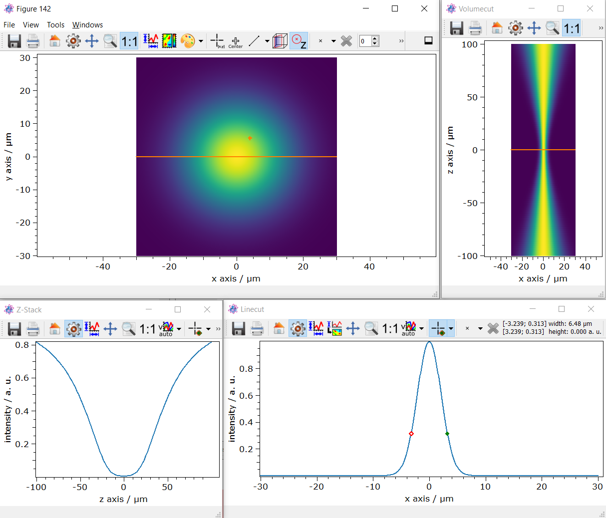
12.1.10.5.19.1. Generate further volume, line plots from the 3D stack.

Per default the z=0 plane is plotted. Above the image there are buttons to cut the 3D stack.

In this 3D stack plot, a sectional view through the volume can now be generated shown in the upper right plot. Furthermore, a line cut between two pixels can be created form this 2D plot shown in the lower right plot.

In this plot, a distance between two pixels can then be calculated by the picker. In this example, the Gaussien width is about 6.47 \u00B5m.

Additionally a line cut through z can be created shown in the lower left plot.

plot(gauss3D, properties={"keepAspectRatio": True, "colorMap": "viridis"})

(145, PlotItem(UiItem(class: Itom2dQwtPlot, name: plot0x0)))