8.2. Array class DataObject
8.2.1. Introduction
In itom, the class dataObject is the main array object. Arrays in itom can have the following properties:
unlimited number of dimensions
each dimension can have an arbitrary size
- possible data types:
"uint8"      #unsigned integer, 8 bit [0,255]
"int8"       #signed integer, 8 bit [-128,127]
"uint16"     #unsigned integer, 16 bit [0,65536]
"int16"      #signed integer, 16 bit [-32768,32767]
"uint32"     #unsigned integer, 32 bit
"int32"      #signed integer, 32 bit
"float32"    #floating point, 32 bit single precision
"float64"    #floating point, 64 bit double precision
"complex64"  #complex number with two float32 components
"complex128" #complex number with two float64 components
"rgba32"     #color format, 4x uint8 values (alpha,r,g,b)
Before giving a short tutorial about how to use the class dataObject, the base idea and concept of the array structure should be explained. If you already now the huge Python module Numpy with its base array class numpy.array, one will ask why another similar array class is provided by itom. The reasons for this are as follows:
The python class
dataObjectis just a wrapper for the itom internal class DataObject, written in C++. This array structure is used all over itom and also passed to any plugin instances of itom. Internally, the C++ class DataObject is based on OpenCV-matrices, such that functionalities provided by the open-source Computer-Vision Library (OpenCV) can be used by itom.The class dataObject should also be used to store real measurement data. Therefore it is possible to add tags and other meta information to every dataObject (like axis descriptions, scale and offset values, protocol entries…).
Usually, array classes (like the class Numpy.array) store the whole matrix in one continuous block in memory. Due to the working principle of every operating system, it is sometimes difficult to allocate a huge block in memory. Therefore, dataObject only stores the sub-matrices of the last two-dimensions in single blocks in memory, while the first n-2 dimensions of the array are represented by one vector in memory, where every cell is pointing to the corresponding sub-matrix (called plane). Using this concept, huger arrays can be allocated without causing a memory error.
Note
In order to realize a compatible version with respect to numpy, matlab… data in a DataObject can also be stored continuously. The basic structure for the data object is the same than in the non-continuous (default) version, but the data of each 2dim-matrix lies continuously in memory and each data-pointer of each matrix just points to the first element of the corresponding matrix in this big data block in memory.
The non-continuous representation has advantages especially in the case of huge data sets, since it is more difficult to obtain a free, big continuous block in memory without reorganizing it than multiple smaller blocks of memory, which can be distributed randomly in memory.
Matrixes with only one or two dimension are automatically stored continuously.
8.2.2. Creating a dataObject
In general, a dataObject is created like any other class instance in Python, hence the constructor of class dataObject is called. For a full reference of the constructor of class dataObject, type
help(dataObject)
In the following example, some dataObjects of different size and types are created. Using these constructors, the content of the created array is arbitrary at initialization:
1 2 3 4 5 6 7 8 9 10 11 12 13 14 15 16 17 18 19 20 21 22 23 24 25 26 27 28 29 | #1. empty dataObject, dimensions: 0, size: []
a = dataObject()
#2. one dimensional dataObject
# a one dimensional dataObject already is
# allocated as an array of size [1 x n]
b = dataObject([5], "float32") #size [1x5]
#3. 5 x 3 array, type: int8
c = dataObject([5,3], "int8")
#4. 2 x 5 x 10 array, type: complex128
# here two planes of size [5x10] are created and a vector with two items points to them
d = dataObject([2,5,10], "complex128")
#5. 2 x 5 x 10 array, type: complex128, continuous
# This matrix has the same size and type than matrix
# 'd' above. However, the continuous keyword indicates,
# that python should already allocate all planes in
# one block. Then the data object can be converted in
# a numpy.array without the need of copying the data block
# in memory. It is useful to use this keyword, if you
# often want to switch between dataObject and numpy.arrays.
# However consider that this is not recommended for huge
# matrices.
e = dataObject([2,5,10], "complex128", continuous = True)
#6. create a 2x3, uint16 dataObject filled with [[1,2,3],[4,5,6]]
f = dataObject([2,3], "uint16", data = (1,2,3,4,5,6))
|
You can also use the copy constructor of class dataObject in order to create a dataObject from another array-like object or a sequence of numbers (tuple, list…). In Python it is usual, that different objects share their memory (for arrays the memory is mainly the data block(s)) as long as possible, such that memory and execution time is saved. This is also the case when using the copy constructor. See the Numpy documentation for more information about this. The main thing you should know is, that if you change the value of any cell of an array, the corresponding value is also changed in all arrays, that share their memory with the dataObject.
1 2 3 4 5 6 7 8 9 10 11 12 13 14 15 16 17 18 | #1. create dataObject from any array-like object (e.g. Numpy array)
import numpy as np
a = np.ndarray([5,7])
b = dataObject(a) #b has the continuous flag set
#2. create dataObject from a tuple of values
# any object, that python can interpret as sequence can be used
# in order to initialize the data object. The dataObject can have
# an arbitrary size or number of dimensions, if the total number
# of elements fits to the length of the given input sequence.
# In this case, the sequence is totally copied into the data object.
# The values are filled row-by-row into the array, also called as
# c-continuous creation.
c = (2,7,4,3,8,9,6,2) #8 values
d = dataObject([2,4], data = c)
#3. create a dataObject as shallow copy of another dataObject
e = dataObject(d)
|
8.2.3. Static constructors for dataObjects
If a dataObject is created using one of the default constructors (without keyword data), the matrix is allocated to the right side but the values usually have no defined content. The values are even not randomly distributed. In order to generate a pre-filled dataObject, there exist some special static methods. These are:
Use
eye()to create a 2D, square, eye matrix.ones()is used to created a n-dimensional dataObject filled with ones.zeros()is used to created a n-dimensional dataObject filled with zeros.rand()is used to created a n-dimensional dataObject filled with uniformly distributed random values: range [0,1) for floating point values, else the values are taken from the entire value range of the data type.randN()is used to created a n-dimensional dataObject filled with gaussian distributed random values.
a = dataObject.ones([3,4], 'uint8')
a.data()
#returns:
#dataObject(size=[3x4], dtype='uint8'
#    [[  1,   1,   1,   1],
#     [  1,   1,   1,   1],
#     [  1,   1,   1,   1]])
8.2.4. Print content of dataObject
If you type the variable name of a dataObject into the command line of itom and press return, the short string representation with all important
facts of the dataObject are printed in one line. This is the same result than using the print() command of Python. If you want to obtain
the full content of a dataObject in the command line, use the method data():
a = dataObject.ones([3,4], 'uint8')
print(a)
#returns:
#dataObject('uint8', [3 x 4], continuous: 1, owndata: 1)

a.data()
#returns:
#dataObject(size=[3x4], dtype='uint8'
#    [[  1,   1,   1,   1],
#     [  1,   1,   1,   1],
#     [  1,   1,   1,   1]])
Note
The string representation (using the print() method) of a numpy array will print the full or cropped content of the numpy array
to the command line (cropped if it is too big). For dataObjects, the content is only print using the data() method.
8.2.5. Accessing values in a dataObject
In order to read or write single values of a dataObject, use the indexing operator:
a = dataObject.ones([2,3], 'uint8')
print("first element", a[0,0])
print("last line:", a[1,0], a[2,0], a[3,0])
#write 5 to the first value:
a[0,0] = 5
The index operator obtains n comma separated arguments, one for each axis. Each index starts with 0, the order of axes is y,x, z,y,x, …
A dataObject is an iteratible object in Python, like lists, tuples, numpy.arrays, … Therefore, it is possible to iterate through all values of a dataObject, whereas the iterator at first goes along the last axis (x), then along the second axis (y) and so on:
a = dataObject([2,3,2], 'uint8', data=(1,2,3,4,5,6,7,8,9,10,11,12))
a.data()

'''returns:
dataObject(size=[2x3x2], dtype='uint8'
[0,:,:]->([[  1,   2],
       [  3,   4],
       [  5,   6]])
[1,:,:]->([[  7,   8],
       [  9,  10],
       [ 11,  12]])
'''

for val in a:
    print(a)

'''returns:
1,2,3,4,5,6,7,8,9,10,11,12
'''
All fixed-point data types are represented by the python type int, all real floating point data types by float, the complex data types by complex and
the color type by rgba.
It is not only possible to address single values within a dataObject, but the index (or mapping) operator also allows the usage of slices. Then, sub-regions of dataObjects can be returned in terms of another dataObject instance. However, it is very important to mention, that a slice or sub-region shares its data memory with the original object. Once you change one value in the original or sliced object, the corresponding value is also changed in all related objects. This is the main philosophy of Python and also holds for numpy.arrays.
Considering slices, the index of any axis in the indexing or mapping operator can then have the following forms:
single, zero-based integer value: Only the one value in the corresponding axis is addressed
start:end: A range of values in the corresponding axis is addressed, where start is the first, zero-based index that is included in the range and end is the last value that is NOT part of the range (excluded).
colon operator (:): All values in this axis are addressed.
a = dataObject.ones([10,20,15])

#get subpart
b = a[5:10, :, 0]
#b then has the size [5,20,1]

#set all values in b to 0:
b[:,:,:] = 0
print(a[4,0,0]) #-> 1
print(a[5,0,0]) #-> 0
print(b[0,0,0]) #-> 0
8.2.6. Basic attributes of a dataObject
Any created dataObject provides some basic attributes that describe the corresponding array:
The attribute
ndimordimsreturn the number of dimensions of the dataObject.The attribute
shapereturns a tuple with the size for every axis. The size of the tuple corresponds to the number of dimensions. Remember, that the order is always (y,x), (z,y,x)…The attribute
dtypereturns a string with the type of the dataObject (e.g. uint8, float32 or complex64).The attribute
continuousreturns True if the data block lies continuously in memory or not (False). False is only possible for 3 or higher dimensional dataObjects. Then, the memory of the single planes lies distributed at different locations in the memory allowing to save bigger matrices in the available memory. While a continuous dataObject can share its memory with a numpy array, a non-continuous dataObject has to be converted in the continuous version before being transmitted to a numpy array (this is implicitely done).
Examples:
a = dataObject.ones([5,4,3,2], 'uint16')
print("dims:", a.ndim, "shape:", a.shape, "type:", a.dtype)
#returns:
#dims: 4 shape: (5, 4, 3, 2) type: uint16
8.2.7. Value and axes descriptions, units, scaling and offset
Usually, dataObjects and numpy arrays are quite similar and very compatible to each other. They can even share memory (if continuous) and dataObjects can usually be
used whenever a function requires an array-like input type (the class dataObject implements the array-like interface definitions). However, the
dataObject has been made in order to also save protocol information, meta information as well as the physical meaning of the matrix. As one powerful feature, it is possible
to set an arbitrary description, unit, scaling and offset to all axes as well as a description and unit to the values. If a dataObject is plot (e.g. by itom.plot()),
these properties are read and considered in the plot.
In detail:
Every axis as well as the value axis can have a description (e.g. ‘length’)
Every axis as well as the value axis can have a unit (e.g. ‘mm’, ‘m’, ‘nm’…). Some algorithms consider these units for special calculations.
Every axis (but not the value axis) can have a scaling (default: 1.0)
Every axis (but not the value axis) can have an offset (default: 0.0)
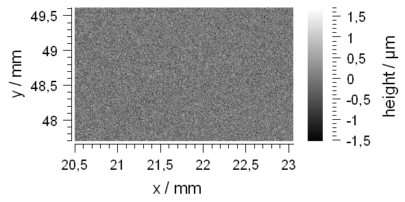
Scaling and offset transform the pixel coordinate in the matrix (beginning with 0 in all axes) into a physical coordinate. While the values in a matrix are always addressed by their pixel coordinate (in integer values), the physical units are displayed in the plots (e.g. designer widget type itom1dqwtplot or itom2dqwtplot). The following example should explain the advantage of the scaling and offset values:
Lets assume that a white-light interferometer records a 2.5D topography of an object. The distance between two adjacent pixels in 2.5 µm in both directions. Additionally, the start position of the x-y-stage is (20.5 mm and 47.7 mm in x and y direction, respectively). These values can then be considered in the obtained dataObject by the following code:
# coding=iso-8859-15
# the coding is important due to the micron sign below

record = dataObject.randN([768, 1024], 'float32')
#record is assumed to be a dataObject
record.axisScales = (0.0025, 0.0025)
record.axisOffsets = (-47.7 / 0.0025, -20.5 / 0.0025) #offset is given in pixel
record.axisUnits = ('mm', 'mm')
record.axisDescriptions = ('y', 'x')
record.valueUnit = ('µm')
record.valueDescription = 'height'
plot(record)
The output is then:
The relation between pixel coordinates and the physical coordinates is:
phys = (pix - offset) * scaling
pix = phys / scaling + offset
These transformations can be done using the methods physToPix() and pixToPhys().
8.2.8. Meta tags and protocol
It is often required to store further meta information together with a dataObject. For this purpose, the dataObject provides arbitrary meta tags (either string or double values) or a string based protocol list. While the first can be used to store timestamps, system configurations, calibration states, … the latter can be used to document filter chains that have already be executed.
Tags are always a mapping between a string-keyword and either a double or string value. The class itom.dataObject provides several functions and attributes in order
to set or read tags:
1 2 3 4 5 6 7 8 9 10 11 12 13 14 15 16 17 18 | obj = dataObject([10,10], 'float32')
#add new tags:
obj.setTag("sensor", "confocal sensor v1.0")
obj.setTag("aperture", 0.6)
#get tags:
print("aperture:", obj.tags["aperture"])
print("sensor:", obj.tags["sensor"])
print("num tags:", len(obj.tags))
if obj.existTag("manufacturer"):
print("The tag 'manufacturer' exists")
else:
print("The tag 'manufacturer' does not exist")
#delete tag
success = obj.deleteTag("aperture")
print("success:", success)
|
The output will be:
aperture: 0.6
sensor: confocal sensor v1.0
num tags: 2
success: True
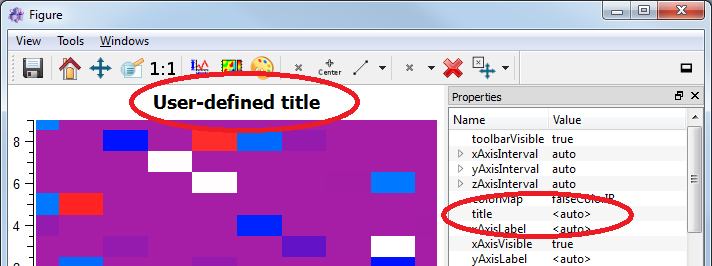
One special tag is the ‘title’-tag. If you plot a dataObject with a string-based ‘title’-tag (e.g. with itom1dqwtplot or itom2dqwtplot), the title tag will be used as title for the plot (if the property title of the plot is set to <auto>):
1 2 | obj.setTag("title", "User-defined title")
plot(obj, "2D")
|
This code will lead to the following plot (under the assumption, that the designer plugin itom2dqwtplot is set as default 2D plot in the properties dialog of itom):
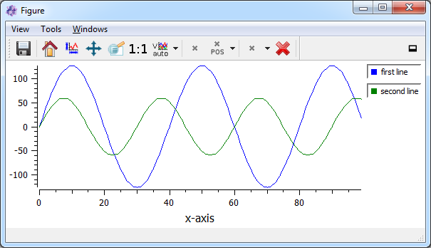
Another special tag is only important for 1D-plots (using the designer plugin itom1dqwtplot). You can then set the legend titles for every single curve. This is done by the tag legendTitleX where X is a continuous line index starting with 0. The following example shows how to create a 2D dataObject with two rows and 100 columns. In the first line (row 0), a sine with an amplitude of 127 is created, in the second line (row 1), a sine with an amplitude of 60. Then, the dataObject is plot as 1D plot (indicated by “1D”) and the property legendPosition is set to Right (per default, no legend is shown):
import math
a = dataObject.zeros([2,100],'int8')
a[0,:] = [127 * math.sin(x * math.pi / 20) for x in range(0,100)]
a[1,:] = [60 * math.sin(x * math.pi / 15) for x in range(0,100)]
a.setTag("legendTitle0", "first line")
a.setTag("legendTitle1", "second line")
plot(a, "1D", properties = {"legendPosition":"Right"})
The result looks like this:
The attribute tags returns a mapping object to a dictionary. This has to be considered to be a read-only dictionary, where no item can be deleted, appended
or changed. However, it is possible to assign a new dictionary to this attribute. Then, all current tags are deleted and the new dictionary items are considered to be the new tags.
The protocol of a dataObject is a list of strings. Use the method addToProtocol() in order to add a new entry to the protocol. If the dataObject is
a slice of another object, the string ROI[…] with the current slice parameters is prepended to each new protocol entry. Finally, the protocol is stored as tag protocol
and can be requested and deleted using the methods described above.
Note
It is not possible to set tags or protocol entries for empty dataObjects. Tags and the protocol is shared between two shallow copies, hence, if two dataObjects share the same data, they also share their tags and protocol.
8.2.9. DataObject vs. Numpy.array
The most common Python package that is used for numeric calculations is Numpy. Numpy is one of the most famous and used Python packages and is the basis
for other packages, like Scipy, Matplotlib, Scikit-image, … Numpy is directly included in itom and also connected to some features of the GUI. Nevertheless,
the main array structure of itom is the class dataObject and not numpy.array. The main reason for this is, that the basis of dataObject
is a C++ class with the same name that can be used in all plugins. Further points for the class dataObject are:
Numpy arrays are always stored in one continuous block in memory. This is a compact and fast structure, however huge matrices can easily run into memory errors, since the computer may have free memory, however probably not in one single block in memory. Therefore, a dataObject usually stores every plane (this is every 2d array of the last two dimensions (x-y-plane)) in one block, whereas all planes lie at arbitrary positions in memory. This is only the case, if the dataObject is created as non-continuous object (see constructor of
dataObject). 2D dataObjects are always continuous.DataObjects are also created with respect to measurement data. Therefore, dataObjects have further meta information, like stated in the sections above.
Internally, every plane in a DataObject is based on OpenCV matrices (in the C++ code). Therefore, it is directly possible to apply OpenCV methods to DataObjects. Furthermore, a direct
use of dataObjects, created in Python, in algorithms or hardware plugins is possible.
Despite the stated differences, the good is, that the classes dataObject and numpy.array are compatible to each other. This is especially the case for continuous dataObjects. They can directly be converted to and from numpy.arrays even as shallow copy, such that both objects share the same matrix memory. If a 3- or higher dimensional dataObject is converted to a numpy-array, it is implicitly converted to a continuous form (such that all planes lie in adjacent blocks in the memory).
Examples for these conversions are:
import numpy as np

dobj2d = dataObject([10,5], 'uint8')
np2d = np.array(dobj2d) #deep copy
np2d_v2 = np.array(dobj2d, copy = False) #shallow copy
dobj2d_v2 = dataObject(np2d) #shallow copy

dobj3d = dataObject([10,20,30], 'uint8') #non-continuous
np3d = np.array(dobj3d, copy = False) #deep copy, since implicit continuous conversion
dobj3d_v2 = dataObject(np3d) #shallow copy of np3d

dobj3d2 = dataObject([10,20,30], 'uint8', continuous = True)
np3d2 = np.array(dobj3d2, copy = False) #shallow copy
dobj3d2_v2 = dataObject(np3d2)
In order to understand these examples, the following things have to be mentioned or repeated: Per default, a dataObject with more than two dimensions is created as non-continuous dataObject, hence various planes (the 2d matrix spanned by the last two axes) are distributed at different locations in memory. If passing a dataObject to the constructor of a numpy.array a deep copy is created per default. Deep copy means, that the array data is entirely copied to another location in memory, such that both arrays are completely de-coupled. This is not the case if the optional parameter copy of the np.array constructor is set to False. If possible, a so called shallow copy is then created such that as little as memory has to be copied. This is the default for most python operations! If both objects are a shallow copy of each other, a change of one value in the one object also changes the other object. However, only values are changed, never types or sizes. A shallow copy is therefore only possible if no change in type or memory structure is required. If a sub-region of an object is copied, a shallow copy is possible. However, this is not the case if the type is changed or if a non-continuous dataObject has to be converted to a numpy.array.
While the copy constructor of a np.array usually creates a deep copy (default setting), the copy constructor of a dataObject always tries to make a shallow copy if possible.
Usually, all methods of Numpy not only work with np.arrays but also with array-like objects. These are python objects that provide a specific interface such that Numpy can implicitely obtain a Numpy array out of them. This is also what dataObject provides. Therefore you can pass every dataObject to a numpy function without a previous conversion to a numpy array.
On the other side, itom often supports numpy arrays without conversion to dataObject. This is for instance the case for the method itom.plot(). Only, when passing arrays
to algorithm or hardware plugins (classes dataIO or actuator, method filter()), usually numpy.arrays have to be converted to
dataObjects:
import numpy a np
import itom

a = np.array([[1,2,3],[4,5,6]])
itom.plot(a) #works
itom.filter("minValue", a) #raises an error
itom.filter("minValue", itom.dataObject(a)) #works
8.2.10. Main operations on numpy.arrays and itom.dataObjects
The following list in an extract of the itom cheatsheet (http://itom.bitbucket.io/media.html) and shows major operations on numpy.arrays and itom.dataObjects:
np.array (import numpy as np) |
itom.dataObject (import itom) |
|
|---|---|---|
arr=np.ndarray([2,3],’uint8’) |
dObj = dataObject([2,3],’uint8’) |
create a randomly filled 2x3 array with type uint8 |
arr=np.array([[1,2,3],[4,5,6]]) |
dObj =dataObject([2,3],data=(1,2,3,4,5,6)) |
create the 2x3 array [1,2,3 ; 4,5,6] |
arr=np.array(dObj, copy = False) |
dObj =dataObject(arr) |
convert np.array <-> dataObject (shallow copy if possible) |
arr.ndim |
dObj.ndim |
Returns number of dimensions (here: 2) |
arr.shape |
dObj.shape |
Returns size tuple (here: [2,3]) |
arr.shape[0] |
dObj.shape[0] |
Returns size of first dimensions (here: y-axis) |
c=arr[0,1]; arr[0,1]=7 |
dObj[0,1]; b[0,1]=7 |
Gets or sets the element in the 1st row, 2nd col |
c=arr[:,1:3] or |
c=dObj[:,1:3] or |
Returns shallow copy of array containing the 2nd and 3rd columns |
c=arr[0:2,1:3] |
c= dObj [0:2,1:3] |
|
arr[:,:]=7 |
dObj[:,:]=7 |
sets all values of array to value 7 |
arr.transpose() (shallow copy) |
dObj.trans() (deep copy) |
transpose of array |
np.dot(arr1,arr2) |
dObj1 * dObj2 (float only) |
matrix multiplication |
arr1 * arr2 |
dObj1.mul(dObj2) |
element-wise multiply |
arr1 / arr2 |
dObj1.div(dObj2) |
element-wise divide |
arr1 +,- arr2 |
dObj1 +,- dObj2 |
sum/difference of elements |
arr1 +,- scalar |
dObj1 +,- scalar |
adds/subtracts scalar from every element in array |
arr1 &,| arr2 |
dObj1 &,| dObj2 |
element-wise, bitwise AND/OR operator |
arr2 = arr1 |
dObj2 = dObj1 |
referencing (both still point to the same array) |
arr2 = arr1.copy() |
dObj2 = dObj1.copy() |
deep copy (entire data is copied) |
arr2 = arr1.astype(newtype) |
dObj2 = dObj1.astype(‘newtypestring’) |
type conversion |
arr = np.zeros([3,4],’float32’) |
dObj = dataObject.zeros([3,4], ‘float32’) |
3x4 array filled with zeros of type float32 |
arr = np.ones([3,4],’float32’) |
dObj = dataObject.ones([3,4], ‘float32’) |
3x4 array filled with ones of type float32 |
arr = np.eye(3,dtype=’float32’) |
dObj = dataObject.eye(3, ‘float32’) |
3x3 identity matrix (type: float32) |
arr2 = arr1.squeeze() |
dObj2 = dObj1.squeeze() |
converts array to an array where dims of size 1 are eliminated (deep copy if necessary) |
np.linspace(1,3,4) |
4 equally spaced samples between 1 and 3, inclusive |
|
[x,y] = np.meshgrid(0:2,1:5) |
two 2D arrays: one of x values, the other of y values |
|
np.linalg.inv(a) |
inverse of square matrix a |
|
x=np.linalg.solve(a,b) |
solution of ax=b (using pseudo inverse) |
|
[U,S,V] = np.linalg.svd(a) |
singular value decomposition of a (V is transposed!) |
|
np.fft.fft2(a), np.fft.ifft2(a) |
filter available (Inverse) 2D fourier transform of a |
|
a[a>0]=5 |
a[a>0] = 5 |
sets all elements > 0 of a to 5 |
a[np.isnan(a)]=0 |
a[np.isnan(a)]=5 |
sets all NaN values of a to 5 |
arr2 = arr1.reshape([3,2]) |
dObj2 = dObj1.reshape([3,2]) |
reshapes arr1 to new size (equal number of items) |
For a detailed methods-summery of the dataObject see itom Script Reference.